The Grubbs’ test#
Purpose#
Grubbs’ test is used to detect a single outlier in a dataset that is assumed to be normally distributed. You need at least three data points.
If you suspect more than one outlier may be present, it is recommended that you use the generalized extreme studentized deviate (ESD) test as the test can be affected by masking. Masking can occur when too few outliers are specified in the test. For example, if you test for a single outlier when there are actually two or more, the additional outliers can influence the test statistic enough that no points are identified as outliers.
How it works#
First, a null hypothesis (\(H_{0}\)) is defined. In this case, H₀ assumes that there are no outliers in the dataset. The alternative hypothesis (\(H_{a}\)) is that there is exactly one outlier in the dataset.
Next, we calculate the Grubbs’ test statistic, G
with \(\overline{Y}\) and s denoting the sample mean and standard deviation, respectively. The Grubbs’ test statistic is the largest absolute deviation from the sample mean in units of the sample standard deviation.
This is the two-sided version of the test. The Grubbs’ test can also be defined as one of the following one-sided tests:
test whether the minimum value is an outlier
\[ G = \frac{\overline{Y}-Y_{min}}{s} \]with \(Y_{min}\) denoting the minimum value.
test whether the maximum value is an outlier
\[ G = \frac{Y_{max}-\overline{Y}}{s} \]with \(Y_{max}\) denoting the maximum value.
For the two-sided test, the hypothesis of no outliers is rejected if \(G > G_{critical}\), the Grubbs’ critical value
with \(t_{\alpha/(2N),N-2}\) denoting the critical value of the t distribution with (N-2) degrees of freedom and a significance level of α/(2N).
For one-sided tests, we use a significance level of α/N.
Example: one-sided Grubbs’ test#
# Import the libraries needed

import matplotlib.pyplot as plt   # For creating visualizations and plots
import numpy as np                # For numerical computations and handling arrays
import scipy.stats as stats       # For statistical functions and probability distributions
# Define an example dataset

# Create a 1D NumPy array with some sample values (our dataset)
y = np.array([0.199, 0.200, 0.200, 0.201, 0.202, 0.203, 0.202, 0.246])

# Create an array with evenly spaced numbers within a given interval (0, 1, 2, ...) to use as the x-axis
# Use np.arange(start (optional, default = 0), stop = len(y), step (optional, default = 1))
x = np.arange(len(y))
# Visualize the dataset

# Create a scatter plot of the data using x = indices (0, 1, 2, ...) and y = dataset values
plt.scatter(x,y)

# Add labels to the x-axis and y-axis
plt.xlabel("Index (x)")         # Describes what x-values represent
plt.ylabel("Data values (y)")   # Describes what y-values represent

# Add a title to the plot
plt.title("Scatter Plot of Example Dataset")

# Display the plot
plt.show()
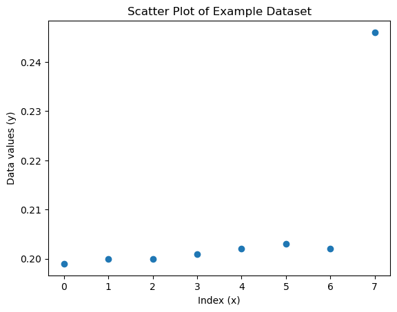
Most values are very close together (between 0.199 and 0.203). Then suddenly, there’s a jump to 0.246. This makes it a potential outlier. Let’s apply a one-sided Grubbs’ test.
Null hypothesis (\(H_{0}\)): there are no outliers in the data
Alternative hypothesis (\(H_{a}\)): the maximum value is an outlier
The null hypothesis of no outliers is rejected if \(G > G_{critical}\) .
# Step 1: Calculate Grubbs' test statistic, G

mean_y = np.mean(y)                   # Mean of the dataset
std_y = np.std(y, ddof=1)             # Sample standard deviation (ddof=1 for sample (N-1), not population (N))
abs_diff = np.abs(y - mean_y)         # Absolute differences of each dataset value from the mean
max_abs_diff = np.max(abs_diff)       # Largest absolute difference from the mean
G_calculated = max_abs_diff / std_y   # Largest deviation divided by sample standard deviation, Grubbs' test statistic G
# Step 2: Calculate the critical value

# Define a function to calculate the Grubbs critical value using sample size and significance level
def calculate_critical_value(size, alpha):
    """
    Calculate the critical value using the formula given in NIST's Grubbs' Test for Outliers

    Arguments:
        size (int): sample size of the dataset (n)
        alpha (float): significance level (commonly 0.05 for 5%)

    Returns:
        critical value (float): the critical value for this sample size and significance level
    """
    t_crit = stats.t.ppf(alpha / (2 * size), size - 2)                                            # Critical value for two-tailed test
    critical_value = ((size - 1) / np.sqrt(size)) * np.sqrt(t_crit**2 / (size - 2 + t_crit**2))   # Formula for Grubbs' critical value

    return critical_value

# Calculate and display the Grubbs critical value for dataset y at 5% significance
# As the function above is for a two-tailed test and we are performing a one-tailed test, we need a signifinace level of 10%.
G_critical = calculate_critical_value(len(y), 0.1)
# Step 3: Compare and interpret results

# Print the Grubbs' test statistic (G_calculated) and the Grubbs' critical value (G_critical) rounded to 3 decimal places ({:.3f})
# Use format() to embed variables directly in a string
print("Grubbs' test statistic (G): {:.3f}".format(G_calculated))
print("Grubbs' critical value (G_critical): {:.3f}".format(G_critical))

# Compare the Grubbs' test statistic with the critical value
if G_calculated > G_critical:
    # If the calculated value is larger than the critical value, the extreme point is an outlier
    print("Reject the null hypothesis. An outlier is detected.")
else:
    # If the calculated value is smaller or equal, no significant outlier is detected
    print("Accept the null hypothesis. No outlier detected.")
Grubbs' test statistic (G): 2.467
Grubbs' critical value (G_critical): 2.032
Reject the null hypothesis. An outlier is detected.
Resources#
Grubbs, F. E. (1969). Procedures for Detecting Outlying Observations in Samples. Technometrics, 11(1), 1–21. Available here.
National Institute of Standards and Technology (NIST), Grubbs’ Test for Outliers. Available here.
Bhavesh Bhatt, Grubbs’ Test for Outlier Detection using Python. Available here.
GraphPad, Detecting outliers with Grubbs’ test. Available here.